E2E GenFirst

GenFirst

Generation Before Reconstruction for
Stable End-to-End Latent Generative Modeling

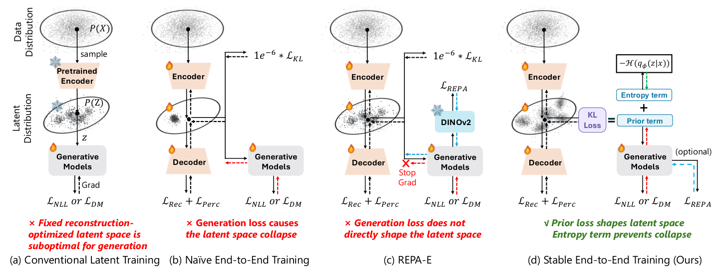
The general framework for stable direct end-to-end training of VAEs and generative models: mapping the data distribution to the distribution modeled by the generative model.

Guangting Zheng1,2, Yiyuan Zhang2, Tao Yang2, Yunpeng Chen2, Rui Zhu2,†, Jiajun Deng1, Yanyong Zhang1,‡
1University of Science and Technology of China 2ByteDance Seed
Project lead · Corresponding author
ByteDance Seed Project
0.97 gFID, ImageNet 256
with guidance
1.45 gFID, ImageNet 256
without guidance
0.90 GenEval overall
text-to-image, 1.3B
≥70× fewer training steps
than SiT at equal FID
Abstract

Can a VAE and its generative prior be trained together, directly?

Latent generative models typically follow a two-stage pipeline, training a variational autoencoder for reconstruction and then a generative model on the frozen latent space. Since reconstruction-optimized latents are not necessarily generation-friendly, jointly training both models is an appealing alternative. However, direct end-to-end training remains challenging, as it is prone to latent collapse and faces a generation–reconstruction conflict.

In this work, we revisit this problem by analyzing how different objectives shape the latent space and identify two key insights. First, the entropy term in the KL objective is essential for preventing collapse: reconstruction and prior fitting both tend to shrink the posterior, while entropy preserves non-degenerate latent uncertainty. Second, reconstruction and generation exhibit asymmetric learning dynamics: reconstruction is fast and strongly supervised, whereas generation is slower and harder to optimize.

Motivated by these insights, we achieve the first direct end-to-end training without latent collapse and further propose GenFirst, a simple generation-before-reconstruction strategy. The generative objective first shapes the latent space under weak reconstruction pressure, after which reconstruction is progressively strengthened to recover visual details. We validate this strategy with both continuous autoregressive priors with exact likelihoods and SiT priors with implicit likelihoods. With our end-to-end objective and GenFirst, SiT achieves a gFID of 0.97 with CFG and 1.45 without CFG on ImageNet 256×256, while MMDiT reaches a GenEval score of 0.90 on text-to-image generation.

Beyond image generation, we further extend the framework to shared visual latents for generation and representation learning, and to continuous unified text–image generation. These results demonstrate the generality of stable end-to-end latent learning across generative priors and modalities.
Comparison of latent generative modeling paradigms
Figure 1. Comparison of latent generative modeling paradigms. (a) Conventional two-stage methods train the generative model on a fixed, reconstruction-optimized latent space that may be suboptimal for generation. (b) Naive end-to-end training lets the generative loss update the encoder, but causes latent collapse. (c) REPA-E avoids collapse by stopping the generative gradient and reshaping the latent space with an external representation-alignment loss, so the generative objective never directly shapes the latents. (d) Our method enables direct end-to-end training: the prior loss shapes a generation-friendly latent space while the entropy term prevents collapse.
Analysis

Two insights behind stable end-to-end training

We revisit end-to-end training from the VAE objective rather than from the architecture, and find that both failure modes reported in prior work have a concrete, correctable cause.

Insight 1 · why it collapses

A prior–entropy imbalance, not a broken gradient

For a standard Gaussian reference prior, the KL regularizer splits into a prior-fitting term and a negative posterior-entropy term:

\[ D_{\mathrm{KL}}(q_\phi(z|x)\|p_0(z)) = \underbrace{\mathbb{E}_{q_\phi}[-\log p_0(z)]}_{\text{prior fitting}} \;-\; \underbrace{\mathcal{H}(q_\phi(z|x))}_{\text{entropy}} \]

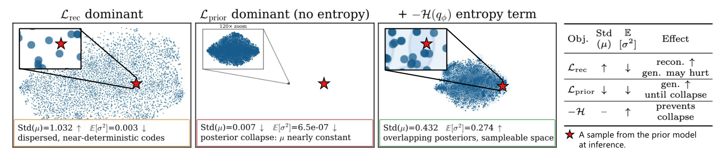
Naive end-to-end training inherits the LDM recipe of a tiny KL weight (\(\lambda_{\mathrm{KL}}\!\approx\!10^{-6}\)) and then adds a learned prior loss on top. The added objective is a strong extra prior-fitting force while entropy stays suppressed: \(\lambda_{\mathrm{prior}}+\lambda_{\mathrm{KL}} \gg \lambda_{\mathrm{KL}}\). Posterior variance is driven to zero, the means concentrate on nearly one code, and the latent space collapses.

The entropy term is not a minor regularizer: it is the counteracting force to learned prior fitting. Making it explicit turns latent collapse from a failure mode into a diagnosable imbalance.
Insight 2 · why weighting is not enough

Reconstruction is fast, generation is slow

Reconstruction is a strongly supervised mapping problem: given latents, the decoder gets direct pixel supervision and recovers detail within few steps. Generation is a distribution-modeling problem: the prior must learn the global latent distribution before it can sample anything recognizable.

Strong reconstruction pressure early therefore anchors the encoder to a reconstruction-oriented latent space that the prior can never catch up with, while permanent generative pressure prevents detail recovery. What matters is not only how the two objectives are weighted, but when each of them shapes the latent space.

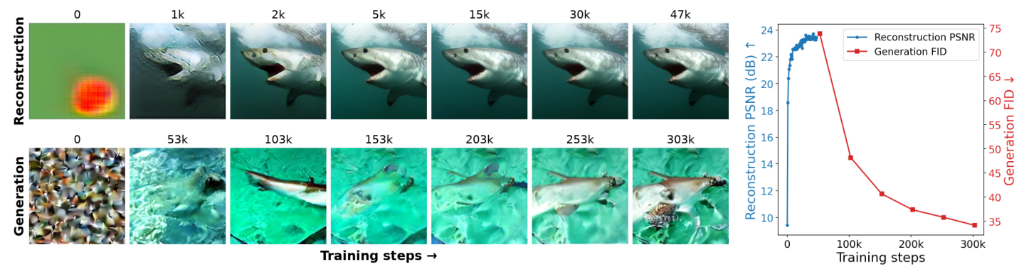
Asymmetric learning dynamics between reconstruction and generation
Figure 2. Reconstruction reaches good fidelity within far fewer steps, while generation needs a much longer optimization process to become sampleable.
Qualitative effects of each objective on the latent posterior
Figure 3. What each objective does to the posterior. Reconstruction spreads the posterior means (\(\mathrm{Std}(\mu)\!\uparrow\)) but shrinks the uncertainty (\(\mathbb{E}[\sigma^2]\!\downarrow\)), leaving gaps between codes that are hard to sample. Prior fitting without entropy shrinks both and collapses the posterior toward a constant code. Adding entropy restores \(\mathbb{E}[\sigma^2]\), increases posterior overlap and makes the latent space sampleable.
Three natural fixes for the generation–reconstruction conflict — none of them works
Latent dimension, VAE size and prior size ablations
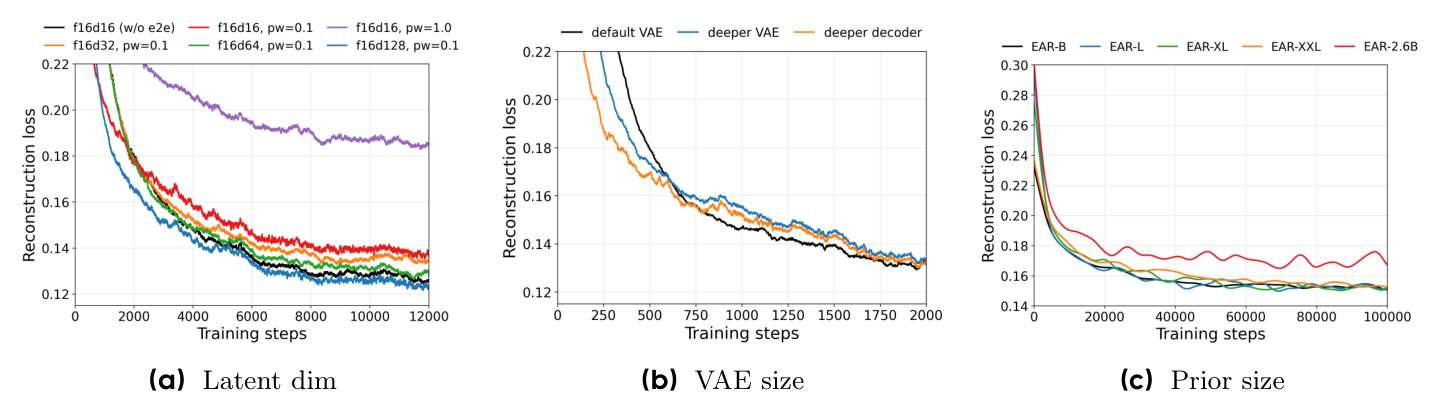
Figure 4. (a) A larger latent dimension tolerates a stronger prior weight, but even \(d\!=\!128\) only supports \(\lambda_{\mathrm{prior}}\!\approx\!0.1\), and makes the AR prior harder to model. (b) Scaling the VAE (deeper encoder/decoder, or decoder only) does not alleviate the conflict and can even hurt reconstruction. (c) Scaling the prior improves generation but pushes reconstruction further down — more shaping pressure, same conflict.
The trade-off of generation and reconstruction
Generation-reconstruction trade-off and GenFirst schedule ablations
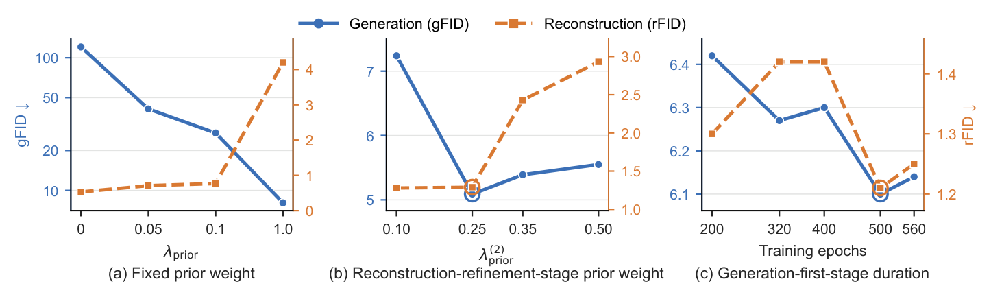
Figure 5. (a) Raising \(\lambda_{\mathrm{prior}}\) from 0 to 1.0 improves gFID from 120.60 to 8.06 while rFID degrades from 0.53 to 4.20 — no fixed weight is favourable for both. (b) In the reconstruction-refinement stage, a moderate prior weight of 0.25 is best. (c) gFID improves with a longer generation-first stage and saturates around 500 epochs.
Table 2. Loss balancing is not enough. Same architecture and budget; only the way the generative objective is controlled differs. Collapsed = NaN training loss.
StrategygFID (w. CFG) ↓IS (w. CFG) ↑ rFID ↓PSNR ↑SSIM ↑
GenFirst (ours)2.10246.701.2621.930.58
Constant weighting3.04251.23.2719.520.48
Cosine decay5.45136.110.6623.870.67
PI adaptive
Frozen VAE (two-stage)6.97147.040.5326.180.72

Constant weighting buys generation at the cost of reconstruction, cosine decay does the opposite, and PI-style adaptive control is numerically unstable in our setting. The optimization order — not the weight schedule — is what resolves the conflict.

Method

An entropy-preserving objective, and generation before reconstruction

One objective makes direct joint training stable; one schedule decides which objective gets to shape the latent space first.

\[ \mathcal{L}_{\mathrm{E2E}} = \lambda_{\mathrm{rec}}\mathcal{L}_{\mathrm{rec}} + \lambda_{\mathrm{LPIPS}}\mathcal{L}_{\mathrm{LPIPS}} + \lambda_{\mathrm{GAN}}\mathcal{L}_{\mathrm{GAN}} + \lambda_{\mathrm{prior}}\mathcal{L}_{\mathrm{prior}} - \lambda_{\mathrm{ent}}\mathcal{H}(q_\phi(z|x)) \]

Prior fitting and posterior entropy are separated and separately weighted. The prior term is whatever generative objective is being trained — an exact latent NLL for the continuous autoregressive prior, or the flow-matching velocity loss for SiT. For SiT we additionally keep the classic \(10^{-6}\) KL term purely to bound the latent scale, since an unbounded \(z\) would make the injected Gaussian noise relatively too small and open another shortcut.

Stage 1

Generation first

A large prior weight (with \(\lambda_{\mathrm{ent}}=\lambda_{\mathrm{prior}}\)) lets the generative objective form a generation-friendly latent geometry, while reconstruction preserves image information and entropy prevents collapse. This stage is the long one: 500 epochs for EAR, 80 epochs for EiT.

Stage 2

Reconstruction refinement

The prior and entropy weights drop together — \(1\!\to\!0.25\) for EAR and \(0.1\!\to\!0.01\) for EiT — giving reconstruction more relative influence so that visual detail returns without dismantling the latent space formed in stage 1. This stage is short: 140 and 40 epochs respectively.

Then

Freeze and train the prior

For diffusion priors the end-to-end phase is followed by a prior-only phase: freeze the learned VAE and train a fresh SiT / MMDiT on its latents. The same frozen VAE also transfers to 512×512 and to text-to-image without retraining the tokenizer.

Instantiation A

EAR — exact-likelihood autoregressive prior

Latents are flattened into \(N=hw\) continuous tokens and modelled by a causal Transformer with a \(K\)-component Gaussian-mixture head, following FARMER: \(p_\theta(z|c)=\prod_i p_\theta(z_i|z_{<i},c)\). The exact likelihood makes the prior–entropy balance directly measurable, and the same loss both fits and reshapes the latent distribution.

Instantiation B

EiT — flow-matching / diffusion prior

SiT for class-conditional ImageNet and MMDiT for text-to-image, trained with the linear-interpolant velocity loss \(\|v_\theta(z_t,t)-(z-\epsilon_t)\|^2_2\). No explicit likelihood over latents is available here, which is exactly why the entropy term (rather than a likelihood diagnosis) is what keeps training stable.

Results

End-to-end latents are easier to generate from

The clearest evidence is not the joint model itself, but what happens when a new prior is trained from scratch on the frozen end-to-end latent space.

Table 1a. EAR. Trained until gFID converges. Collapsed = NaN loss.
SettinggFID ↓IS ↑rFID ↓PSNR ↑SSIM ↑
Frozen VAE36.3346.550.5326.180.72
Naive E2E294.901.480.7025.110.68
Stable E2E (ours)5.10145.221.2621.930.58
Frozen E2E-trained VAE5.67137.391.2621.930.58
Table 1b. SiT (80 epochs). Naive end-to-end training diverges outright.
SettinggFID ↓IS ↑rFID ↓PSNR ↑SSIM ↑
Frozen VAE7.90122.600.7425.670.72
Naive E2E
Stable E2E (ours)92.3813.940.5725.130.71
Frozen E2E-trained VAE3.57166.490.5725.130.71

Replacing a reconstruction-trained VAE with the frozen end-to-end-trained VAE takes a freshly trained prior from 36.33 → 5.67 gFID for EAR and 7.90 → 3.57 for SiT. EAR, whose exact likelihood directly models the VAE density, is slightly better during joint training; SiT, which has no explicit likelihood over latents, prefers the freeze-and-retrain protocol.

Convergence acceleration on class-conditional and text-to-image generation
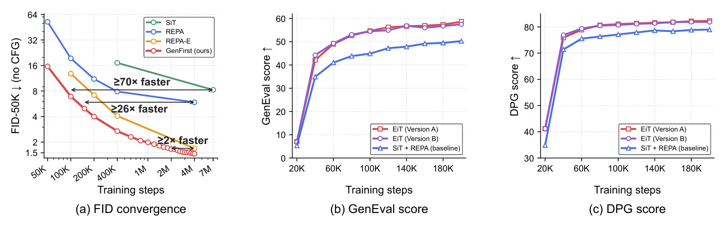
Figure 8. GenFirst latents converge much faster. (a) FID-50K without guidance on ImageNet: GenFirst reaches FID 6.91 at 100K steps and 4.97 at 150K steps, beating the final results of SiT and REPA with at least 70× and 26× fewer steps, and matching REPA-E at roughly lower cost. (b–c) On text-to-image, both EiT variants pass the 200K-step SiT+REPA baseline by 80K steps on GenEval and DPG-Bench.
Class-conditional ImageNet 256×256 — full comparison
Table 6. * results obtained with a low-temperature sampling strategy.
MethodEpochs#Params Without guidanceWith guidance
gFID ↓IS ↑Prec. ↑Rec. ↑ gFID ↓IS ↑Prec. ↑Rec. ↑
Pixel space
ADM400554M10.94101.00.690.633.94215.80.830.53
RIN480410M3.42182.0
PixelFlow320677M1.98282.10.810.60
PixNerd160700M2.15297.00.790.59
SiD212801.38
TARFlow3201.4B4.69
JetFormer5002.8B6.640.690.56
FARMER3201.9B3.60269.20.810.51
JiT6002B1.82292.60.790.62
PixelDiT320797M1.61292.70.780.64
DeCo600682M1.69304.00.790.63
Latent autoregressive
GIVT5001.67B2.590.810.57
VAR3502.0B1.92323.10.820.591.73350.20.820.60
MAR800943M2.35227.80.790.621.55303.70.810.62
xAR8001.1B1.24301.60.830.64
Latent diffusion
DiT1400675M9.62121.50.670.672.27278.20.830.57
MaskDiT1600675M5.69177.90.740.602.28276.60.800.61
SiT1400675M8.61131.70.680.672.06270.30.820.59
MDTv21080675M1.58314.70.790.65
REPA800675M5.78158.30.700.681.29306.30.790.64
VA-VAE800675M2.17205.60.770.651.35295.30.790.65
DDT400675M6.27154.70.680.691.26310.60.790.65
RAE800839M1.51242.90.790.631.13262.60.780.67
End-to-end generative models
SimFlow1601.4B13.72105.20.670.622.15276.80.830.57
REPA-E800675M1.69219.30.770.671.12302.90.790.66
EAR (ours, w/o GenFirst)500312M5.17147.50.700.593.04251.20.730.55
EAR (ours)500+140312M6.10 / 3.83*138.4 / 164.0*0.650.642.10246.70.720.59
EiT (ours)80675M2.79175.40.780.631.38271.30.790.63
EiT (ours)480675M1.60216.80.780.650.988270.70.790.67
EiT (ours)800675M1.45226.70.790.650.969283.40.790.67

EAR reaches a guided gFID of 2.10 with only 312M parameters, outperforming much larger continuous-AR baselines such as GIVT (2.59), FARMER (3.60) and JetFormer (6.64). EiT reaches 0.988 guided gFID after 480 epochs — to our knowledge the first diffusion model below FID 1.0 without a Fréchet-Distance loss — and 1.45 unguided at 800 epochs.

Class-conditional ImageNet 512×512
Table 7. The VAE is trained end-to-end at 256×256, then frozen; only the prior is trained at 512×512.
MethodEpochs#ParamsgFID ↓IS ↑Prec. ↑Rec. ↑
BigGAN-deep158M8.43177.90.880.29
StyleGAN-XL2.41267.80.770.52
VAR3502.3B2.63303.2
MAGVIT-v21080307M1.91324.3
MAR800481M1.73279.9
xAR800608M1.70281.5
ADM871+210731M3.85221.70.840.53
SiD21.50
PixNerd340700M2.84245.60.800.59
JiT6002B1.78306.8
PixelDiT850797M1.81278.60.780.67
DeCo340682M2.22290.00.800.60
DiT600674M3.04240.80.840.54
SiT600674M2.62252.20.840.57
REPA200675M2.08274.60.830.58
Unified Latents1.31
DDT356675M1.28305.10.800.63
EDM21.5B1.25
RAE400839M1.13259.60.800.63
STARFlow1.4B3.00
SimFlow + REPA-E1601.4B2.74304.90.810.57
EAR (ours)320940M1.87280.00.820.58
EiT (ours)80675M1.63278.90.810.61
EiT (ours)400675M1.23286.10.800.63
Comparison with REPA / REPA-E, and how end-to-end training interacts with REPA
Table 4. All models evaluated after 80 epochs.
MethodgFID ↓IS ↑Prec. ↑Rec. ↑
REPA7.90122.600.700.65
REPA-E (scratch)4.34154.300.750.63
REPA-E (SD-VAE init.)4.07161.800.760.62
REPA-E (VA-VAE init.)3.46159.800.770.63
EiT (scratch)3.78161.420.780.61
EiT (SD-VAE init.)3.57166.490.770.62
EiT (VA-VAE init.)2.79175.400.780.63
Scaling the prior, GMM capacity, the optional normalizing flow, and SiT prior weights
Table 3a. EAR model scale on a frozen GenFirst VAE.
Model#ParamsgFID ↓IS ↑
EAR-B174M13.8579.00
EAR-L477M5.67137.39
EAR-XL775M3.91163.71
EAR-XXL1.4B3.19181.99
Table 3b. GMM components with EAR-L fixed.
GMM \(K\)gFID ↓IS ↑
326.08132.70
645.67137.39
1285.64137.24
10245.01144.63
40965.00144.99
Table 5. Is a normalizing flow still needed for continuous AR modeling?
SettinggFID ↓IS ↑
Frozen VAE + AR110.1014.79
Frozen VAE + NF + AR36.3346.55
Stable E2E VAE + AR5.27149.28
Stable E2E VAE + NF + AR5.12151.17
Table 13. GenFirst prior weights for the SiT instantiation.
\(\lambda^{(1)}_{\mathrm{prior}}\)\(\lambda^{(2)}_{\mathrm{prior}}\)rFID ↓PSNR ↑FID ↓IS ↑
1.000.100.6124.574.44154.25
0.100.010.5725.133.57166.49
0.010.010.4825.173.84161.40

After end-to-end training the extra normalizing flow becomes largely optional (5.27 → 5.12), whereas on a frozen reconstruction-optimized VAE it is worth 74 FID points. The latent space produced by GenFirst is already well suited to continuous AR modeling.

What end-to-end training costs in reconstruction
Table 12. VAE reconstruction on ImageNet-256. End-to-end training reshapes the latent space toward generation at a moderate, predictable reconstruction cost.
VAErFID ↓PSNR ↑SSIM ↑LPIPS ↓
FLUX.1-dev VAE0.1831.590.900.05
E2E-trained (Version A: SiT-XL/2 on ImageNet, FLUX.1-dev init.)0.2329.430.850.07
E2E-trained (Version B: MMDiT-L/2 on T2I, FLUX.1-dev init.)0.2129.370.850.07
SD-VAE0.7425.670.720.13
E2E-trained (f8d4, SD-VAE init.)0.5725.130.710.14
VA-VAE0.2826.320.760.11
E2E-trained (f16d32, VA-VAE init.)0.3625.820.740.12
Text-to-image

0.90 GenEval with a 1.3B MMDiT

The end-to-end phase produces a VAE — either with SiT-XL/2 on ImageNet (Version A) or with an MMDiT-L/2 on the text-to-image mixture (Version B). The prior-only phase then trains the same MMDiT-XL/2 on its latents at 256×256 for 200K steps, 512×512 for 80K steps, plus 40K steps of fine-tuning.

Table 8. GenEval and DPG-Bench. uses prompt rewriting; * replaces the CLIP text encoder with Qwen3-1.7B.
Method#ParamsSingleTwo obj.Count ColorPositionAttr.GenEval ↑DPG-Bench ↑
PixArt4.3B+0.6B0.980.500.440.800.080.070.4871.11
DALL·E 20.940.660.490.770.100.190.52
Show-o1.3B0.950.520.490.820.110.280.53
Emu3-Gen8B0.980.710.340.810.170.210.5480.60
SDXL0.81B+2.6B0.980.740.390.850.150.230.5574.65
Janus1.3B0.970.680.300.840.460.420.6179.68
JanusFlow1.3B0.970.590.450.830.530.420.6380.09
FLUX.1 [dev]4.8B+12B0.980.810.740.790.220.450.66
DALL·E 30.960.870.470.830.430.450.6783.50
SD3-Medium5.5B+2B0.990.940.720.890.330.600.7484.08
Show-o2-7B7B1.000.870.580.920.520.620.7686.14
MetaQuery-XL7B0.8082.05
Janus-Pro-7B7B0.990.890.590.900.790.660.8084.19
Z-Image-Turbo4B+6B1.000.950.770.890.650.680.8284.86
BLIP3-o-8B8B0.8481.60
FLUX.2 [dev]24B+32B1.000.990.790.930.730.780.8787.57
Qwen-Image7B+20B0.990.920.890.880.760.770.8788.32
BAGEL-7B7B0.980.950.840.950.780.770.88
EiT (ours)0.1B+1.3B1.000.940.830.940.870.820.9082.60
EiT (ours)*1.7B+1.3B0.990.940.730.960.890.840.8984.65

With 1.3B generation parameters, EiT outperforms much larger text-to-image systems on GenEval, with the largest margins on position (0.87) and attribute binding (0.82). Swapping CLIP for a Qwen3-1.7B text encoder trades a little counting accuracy for +2.05 DPG-Bench.

Same MMDiT, same data — only the VAE differs

Hover a sample (or flip the switch) to swap between the FLUX.1-dev VAE and our end-to-end trained VAE. Click to open it full size; use ←/→ to browse.

Show:
Extension experiment 1 — Shared latents

Toward a shared latent space for generation and representation learning

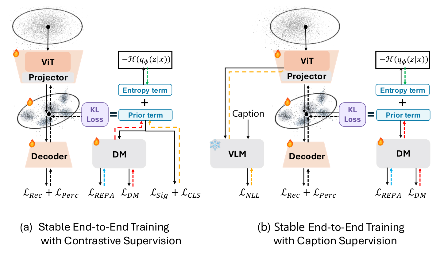
The first of two extension experiments that push the same recipe past text-to-image. If the generative objective can shape a latent space, representation learning can share it. We swap the FLUX.1-dev encoder for a Qwen3-VL ViT plus a posterior projector and add representation supervision inside the same end-to-end loop, so the features being aligned are exactly the latents the diffusion model consumes.

Two ways of adding representation supervision to end-to-end training
Figure 9 (a–b). Two ways to add representation supervision. (a) Latent-level SigLIP supervision, so representation learning shapes exactly the latents the generative model uses. (b) Caption-based VLM-NLL supervision applied to the intermediate ViT features: they are fed to a frozen Qwen3-VL and the caption NLL is minimized — no in-batch negatives needed.
Table 9. Reconstruction, generation and representation quality of different visual encoders. The FLUX.1-dev encoder is replaced by the Qwen3-VL ViT plus a posterior projector; Top-1 is an ImageNet linear probe.
EncoderSettingrFID ↓PSNR ↑GenEval ↑DPG-Bench ↑Top-1 Acc. ↑
FLUX.1-dev VAEPretrained0.1831.593.1
Qwen3-VL ViTPretrained79.64
Qwen3-VL ViT + projectorE2E0.4227.790.8983.7077.71
Qwen3-VL ViT + projectorE2E + SigLIP supervision0.3927.640.9083.7679.25
Qwen3-VL ViT + projectorE2E + VLM-NLL supervision0.4627.190.8983.4981.69

Representation supervision can be folded into end-to-end training almost for free: caption-based VLM-NLL supervision lifts linear-probe accuracy from 77.71 to 81.69, which even exceeds the pretrained Qwen3-VL ViT’s 79.64, while GenEval and DPG-Bench stay at 0.89 / 83.49.

Generation and representation learning can live in one latent space — no separate tokenizer for the diffusion model and no frozen encoder for the probe.
Extension experiment 2 — Unified MMDiT

Unified text-image modeling via an end-to-end diffusion

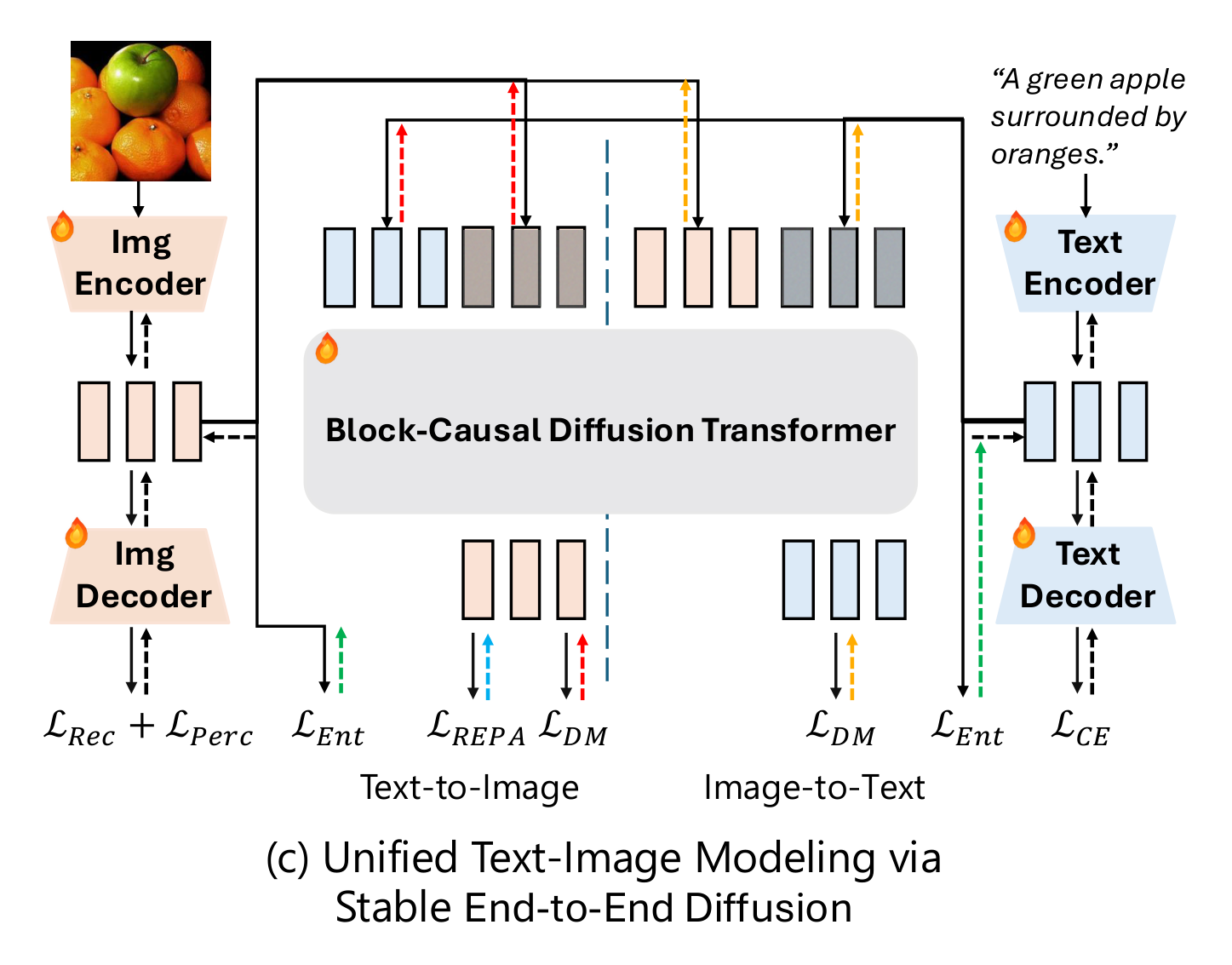
The second extension experiment shows the framework is not tied to pixels. Here we replace one modality outright: text is encoded into continuous latents as well, and a single block-causal MMDiT learns both directions between the two latent spaces.

Unified text-image modeling via end-to-end diffusion
Figure 9 (c). Unified text–image modeling with a block-causal diffusion transformer. Continuous text and image latents are jointly optimized for bidirectional text-to-image and image-to-text generation; entropy terms keep either latent space from collapsing while reconstruction losses keep both decodable.
Setup

Two latent spaces, one diffusion backbone

Text is encoded into continuous latents by a text VAE (initialized from Cola) and reconstructed with a CE loss; text and image latents then enter a block-causal MMDiT trained on \(p(i|t)\) and \(p(t|i)\) with equal probability. Both diffusion directions shape the latent representations, the entropy term prevents collapse, and GenFirst balances latent modeling against reconstruction. Following the text-to-image recipe, the end-to-end phase uses a block-causal MMDiT-L/2 (24 blocks, width 1024) and the prior-only phase trains a fresh block-causal MMDiT-XL/2 (28 blocks, width 1152) from scratch. Because of compute limits, the end-to-end phase uses half the steps of our text-to-image run and the prior-only phase only 30.8% of its samples.

Table 10. Frozen versus end-to-end trained text/image VAEs, with the same block-causal MMDiT and the same three-stage recipe. Image-to-text is evaluated on the COCO Karpathy test split with pycocoevalcap.
SettingGenEval ↑DPG-Bench ↑ CIDEr ↑BLEU-4 ↑METEOR ↑ROUGE-L ↑SPICE ↑CLIPScore ↑
Frozen text VAE + frozen image VAE79.8863.9620.035.3613.7229.018.0353.21
E2E-trained text VAE + frozen image VAE81.8768.2430.197.4616.8132.9511.1255.96
E2E-joint-trained text VAE and image VAE86.5772.6833.287.7617.7434.1611.8157.97

Both arms use the same MMDiT and the same sampling configuration, so the gaps come entirely from how the latent spaces were trained.

Qualitative comparison of the three latent-space settings
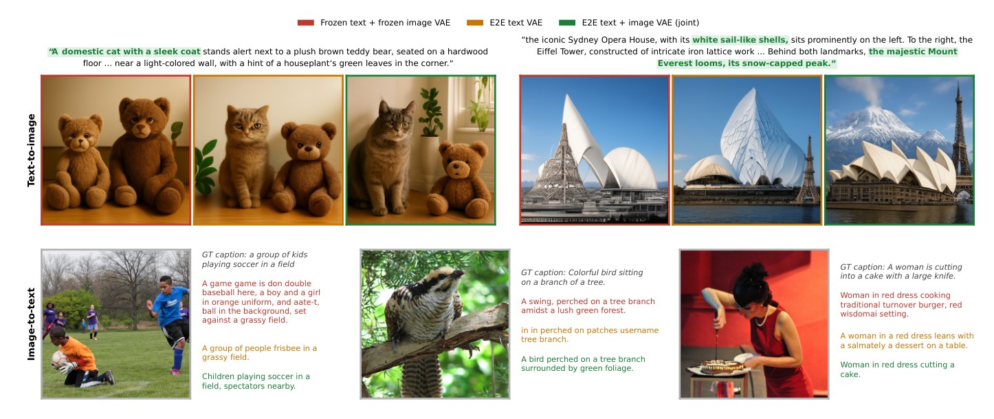
Figure 10. The three latent-space settings, same MMDiT and sampling configuration. Top: text-to-image on DPG-Bench — only the jointly trained latents render the cat rather than a third teddy bear, and place the Opera House, Eiffel Tower and a snow-capped Everest together. Bottom: image-to-text on the COCO Karpathy test split — captions go from incoherent to “children playing soccer in a field”.
Shaping the text latent space end-to-end is worth +1.99 GenEval and +10.2 CIDEr on its own; shaping both latent spaces jointly adds another +4.70 GenEval, +4.44 DPG-Bench and +3.1 CIDEr.
Samples

Class-conditional ImageNet generation

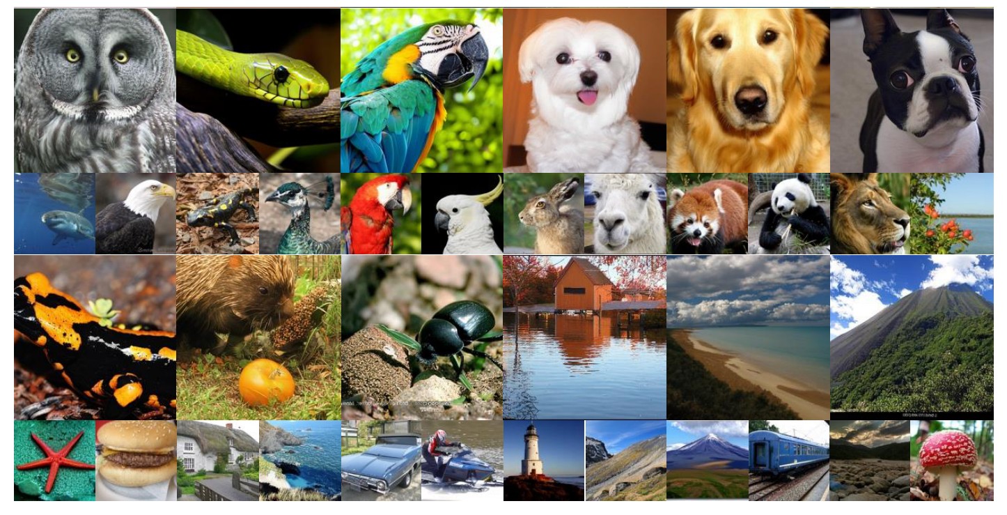
Uncurated samples with guidance from EiT (480 epochs) and EAR (640 epochs) at 256×256. Click any block to view it full size; use ←/→ to browse.

Class-to-image samples from EiT and EAR
Figure 6. Class-to-image samples from EiT (rows 1–2) and EAR (rows 3–4) with guidance, CFG scale 4.
Cite

BibTeX

@article{zheng2026genfirst,
  title   = {GenFirst: Generation Before Reconstruction for Stable
             End-to-End Latent Generative Modeling},
  author  = {Zheng, Guangting and Zhang, Yiyuan and Yang, Tao and
             Chen, Yunpeng and Zhu, Rui and Deng, Jiajun and
             Zhang, Yanyong},
  journal = {arXiv preprint},
  year    = {2026}
}
@inproceedings{zheng2026farmer,
  title={Farmer: Flow autoregressive transformer over pixels},
  author={Zheng, Guangting and Zhao, Qinyu and Yang, Tao and Xiao, Fei and Lin, Zhijie and Wu, Jie and Deng, Jiajun and Zhang, Yanyong and Zhu, Rui},
  booktitle={Proceedings of the IEEE/CVF Conference on Computer Vision and Pattern Recognition},
  pages={25730--25741},
  year={2026}
}

Questions or feedback are very welcome — zgt@mail.ustc.edu.cn.